👀 02 · 图注意力 GAT 与采样邻居 GraphSAGE¶
GCN 给所有邻居同等权重——GAT 用注意力加权,GraphSAGE 用采样+可学习聚合。 本节手写注意力系数(attention score)与加权聚合,再手写 GraphSAGE 的邻居采样与聚合。
🎬 背景故事¶
GCN 给所有邻居等权——可邻居的重要程度明明不同……
GCN 有个小毛病:它给所有邻居平均加权,可你的邻居里,铁哥们和点头之交显然不该同等重要。于是 GAT 引入注意力:让模型自己学每个邻居的权重。而面对超大图,GraphSAGE 又提出另一条路:先采样邻居再聚合。本节把这两个改进逐一实现。
🧭 本节逻辑主线:GCN 等权的局限 → GAT 注意力系数怎么算 → 多头注意力 → GraphSAGE 采样聚合 → 三种聚合器对比 → 怎么选。
📋 本节要解决的问题¶
| # | 问题 | 方法 |
|---|---|---|
| 1 | GAT 与 GCN 区别? | 邻居权重可学习(注意力) |
| 2 | 注意力系数怎么算? | e = LeakyReLU(a[Wh_i ‖ Wh_j]) |
| 3 | GraphSAGE 怎么采样? | 固定大小邻居采样 |
| 4 | 聚合函数有哪些? | Mean / LSTM / Pool |
import matplotlib
import matplotlib.pyplot as plt
matplotlib.rcParams['font.sans-serif'] = ['Microsoft YaHei', 'SimHei', 'PingFang SC', 'Noto Sans CJK SC', 'Arial Unicode MS']
matplotlib.rcParams['axes.unicode_minus'] = False
import numpy as np
import pandas as pd
import networkx as nx
import sqlite3
import os
rng = np.random.default_rng(42)
1️⃣ 构造小图与特征¶
📄 经典论文原图:GAT 注意力与多头机制
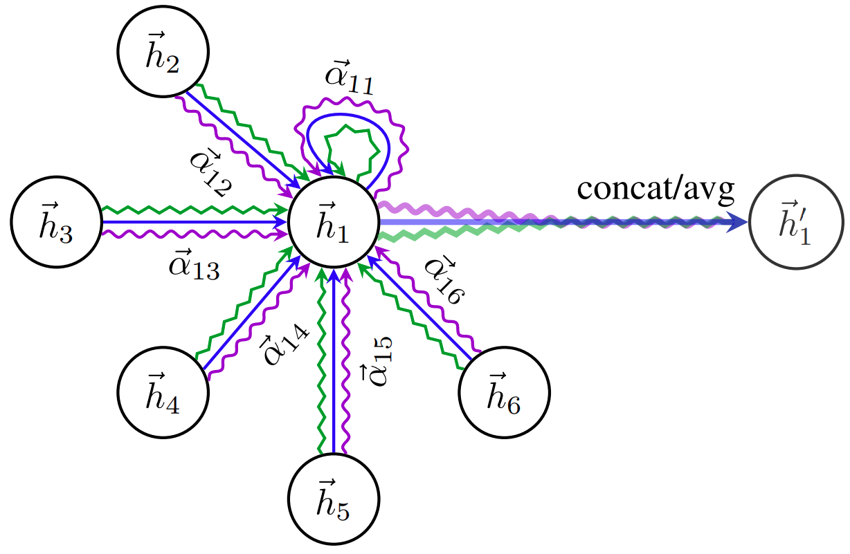
🔍 图解与逻辑衔接:左图展示中心节点如何对邻居计算注意力:先对节点特征做线性变换,再将中心节点与邻居拼接,通过可学习向量和 LeakyReLU 得到未归一化分数,最后 softmax 成注意力系数。右图展示多头注意力:多个独立 attention head 并行聚合邻居,最后拼接或平均,提升模型稳定性和表达能力。它与本节手写的 α 计算逐项对应:左图解释公式,右图解释为什么要多头;后面的 GAT 代码则实现这两个步骤。
论文出处:Veličković et al., “Graph Attention Networks”, ICLR 2018(arXiv:1710.10903),Figure 1。
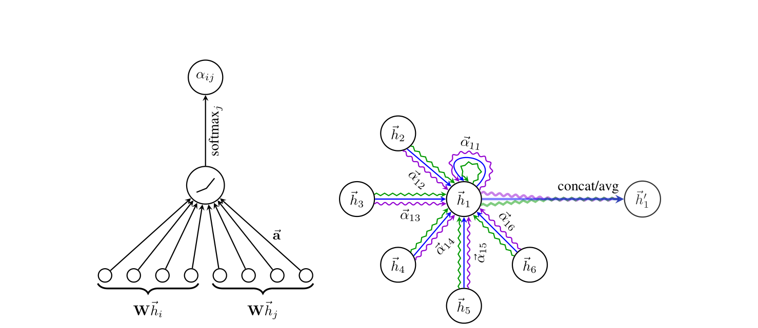
📌 权威配图:GAT 注意力机制图解(GAT 论文一作 Petar Veličković 绘制,Wikimedia Commons,CC BY-SA 4.0)
图中节点 A 的表示由邻居 B/C/D 的注意力加权平均得到——注意力系数 α 是数据驱动的 (按内容学出谁重要),与 GCN 的固定度数先验权重形成鲜明对比。这正是本节手写注意力系数的"原理解释图"。
G = nx.karate_club_graph()
nodes = list(G.nodes())
n = len(nodes)
d = 4
X = rng.normal(0, 1, (n, d))
A = nx.to_numpy_array(G)
print('节点:', n, '特征维度:', d)
print('➡️ GAT 关键差异:给每个邻居算一个可学习权重 α_ij(归一化后和为 1)')
节点: 34 特征维度: 4
➡️ GAT 关键差异:给每个邻居算一个可学习权重 α_ij(归一化后和为 1)
📐 公式推导:GAT 注意力系数与 GraphSAGE 聚合¶
GAT 注意力系数(节点 $i$ 对邻居 $j$ 的重要程度,$\|$ 为拼接、$\mathbf{a}$ 为可学习注意力向量、LeakyReLU 非线性):
$$ e_{ij} = \mathrm{LeakyReLU}\big( \mathbf{a}^\top [ W\mathbf{h}_i \;\|\; W\mathbf{h}_j ] \big), \qquad \alpha_{ij} = \mathrm{softmax}_j(e_{ij}) = \frac{e^{e_{ij}}}{\sum_{k \in \mathcal{N}(i)} e^{e_{ik}}} $$
节点更新(注意力加权聚合 + 非线性;多头时多头输出拼接/取平均):
$$ \mathbf{h}_i' = \sigma\Big( \sum_{j \in \mathcal{N}(i)} \alpha_{ij} \, W \mathbf{h}_j \Big) $$
与 GCN 的区别(推导直觉):GCN 权重 $\frac{1}{\sqrt{\hat{d}_i\hat{d}_j}}$ 是结构先验(按度数固定分配);GAT 权重 $\alpha_{ij}$ 是数据驱动(按内容学出谁重要)。当邻居重要性差异大(如"少数关键用户决定行为")时 GAT 更优。
GraphSAGE 聚合(归纳式:采样 $k$ 个邻居 → 聚合 → 拼接自身,$f$ 为聚合器):
$$ \mathbf{h}_i' = \sigma\Big( W \cdot \big[ \mathbf{h}_i \;\|\; f_{\text{agg}}\big(\{ \mathbf{h}_j : j \in \mathrm{sample}_k(\mathcal{N}(i)) \}\big) \big] \Big) $$
推导要点:① 拼接保留自身与邻居信息(只聚合则自身信息丢失);② 采样固定 $k$ 个邻居把计算量从 $O(\bar{d})$ 压到 $O(k)$,且不依赖全局图(新节点来了直接算)→ 归纳式能力来源;③ GCN 直推式需全图归一化,GraphSAGE 采样使其可处理动态/大规模图。
✍️ §2.1 手算 GAT 注意力系数:两个邻居,谁更值得被关注¶
GAT 注意力 $e_{ij}=\text{LeakyReLU}(a^\top[Wh_i\|Wh_j])$、$\alpha_{ij}=\text{softmax}_j(e_{ij})$——2 节点手算,看"注意力"如何量化邻居权重。
设定:节点 1 特征 $h_1=(1,0)$、节点 2 特征 $h_2=(0,1)$,$W=I$(简化),注意力向量 $a=(1,0,1,0)$。
第 1 步:注意力分数(concat $[h_i\|h_j]$ 然后点乘 $a$)
$$e_{11}=\text{LeakyReLU}([1,0,1,0]\cdot a)=2,\qquad e_{12}=\text{LeakyReLU}([1,0,0,1]\cdot a)=1$$
$$e_{21}=\text{LeakyReLU}([0,1,1,0]\cdot a)=1,\qquad e_{22}=\text{LeakyReLU}([0,1,0,1]\cdot a)=0$$
(LeakyReLU 负斜率 0.2,对 0 输出 0)
第 2 步:softmax 归一化(节点 1 的邻居含自己)
$$\alpha_{11}=\frac{e^2}{e^2+e^1}=\frac{7.389}{10.107}=0.731,\qquad \alpha_{12}=\frac{e^1}{10.107}=0.269$$
第 3 步:聚合
$$h_1'=0.731\cdot Wh_1+0.269\cdot Wh_2=0.731(1,0)+0.269(0,1)=(0.731,\ 0.269)$$
手算收获:
- 注意力分数 $e_{ij}$ 由"$i$ 自己的特征 + $j$ 的特征拼接"经 $a$ 打分——$a$ 是可学习的,决定模型关注哪类模式
- 允许"非对称":$e_{11}=2$ 与 $e_{12}=1$ 不同——节点 1 更关注自己(因为 $a=(1,0,1,0)$ 更匹配"自己"的维度);对比 GCN 的固定平均权重
- 含自环:$\alpha_{ii}$ 也在 softmax 里,GAT 天然把自身作为邻居之一
- softmax 让权重和为 1 且可微——这就是"注意力"替代"平均"做聚合的完整机制(多头 = 多组 $a$ 并行,本 notebook §1 的公式与 §3 的权重对比)
下面 numpy 复算。
# ---- §2.1 验证:numpy 复算 GAT 注意力系数 ----
import numpy as np

h = np.array([[1.0, 0.0], [0.0, 1.0]])
a_vec = np.array([1.0, 0.0, 1.0, 0.0])

def leakyrelu(x, slope=0.2):
    return x if x > 0 else slope * x

def softmax_row(x):
    ex = np.exp(x - x.max())
    return ex / ex.sum()

e = np.array([[leakyrelu(a_vec @ np.concatenate([h[i], h[j]])) for j in range(2)] for i in range(2)])
alpha = np.array([softmax_row(e[0]), softmax_row(e[1])])
print('注意力分数 e =\n', np.round(e, 4))
print('注意力权重 α =\n', np.round(alpha, 4))
assert np.allclose(e, [[2, 1], [1, 0]])
assert np.allclose(alpha[0], [0.7311, 0.2689], atol=1e-3)

h1_new = alpha[0] @ h
print('h1_new =', np.round(h1_new, 4))
assert np.allclose(h1_new, [0.7311, 0.2689], atol=1e-3)
print('\n✓ 与手算一致:注意力权重区分自己与邻居')
2️⃣ 手写注意力系数(单头 GAT,torch)¶
import torch
X_t = torch.tensor(X, dtype=torch.float32)

# 手写 GAT 层:e_ij = LeakyReLU(aᵀ[Wh_i ‖ Wh_j]),softmax over 邻居,加权聚合
class GATLayer(torch.nn.Module):
    def __init__(self, in_dim, out_dim):
        super().__init__()
        self.W = torch.nn.Parameter(torch.randn(in_dim, out_dim) * 0.1)
        self.a = torch.nn.Parameter(torch.randn(2 * out_dim) * 0.1)
        self.leaky = torch.nn.LeakyReLU(0.2)
    def forward(self, H, adj_list):
        Wh = H @ self.W                                    # 线性变换 (n, out)
        outs = []
        for i, nbrs in enumerate(adj_list):
            if not nbrs:
                outs.append(Wh[i])
                continue
            h_i = Wh[i].expand(len(nbrs), -1)              # 广播自己
            e = self.leaky((torch.cat([h_i, Wh[nbrs]], dim=1) @ self.a))  # 注意力分数
            alpha = torch.softmax(e, dim=0)                # 邻居间归一化
            outs.append((alpha.unsqueeze(1) * Wh[nbrs]).sum(dim=0))
        return torch.stack(outs)

adj_list = [list(G.neighbors(i)) for i in nodes]           # 邻居索引(供图操作)
gat = GATLayer(d, 6)
out_gat = gat(X_t, adj_list)
print('GAT 输出形状:', tuple(out_gat.shape))

# 单独演示节点 0 的注意力权重(可学习参数随机初始化)
def attn_alpha0(model, X_t, node=0):
    Wh = X_t @ model.W
    nbrs = adj_list[node]
    h_i = Wh[node].expand(len(nbrs), -1)
    e = model.leaky((torch.cat([h_i, Wh[nbrs]], dim=1) @ model.a))
    return torch.softmax(e, dim=0)

alphas_0 = attn_alpha0(gat, X_t).detach().numpy()
print('节点 0 的邻居注意力权重(前 6 个邻居):')
for j, a in zip(adj_list[0][:6], alphas_0[:6]):
    print(f'  节点 {j}: α = {a:.3f}')
assert np.allclose(alphas_0.sum(), 1)
print('✅ 注意力系数归一化和为 1(softmax over 邻居)')
GAT 输出形状: (34, 6)
节点 0 的邻居注意力权重(前 6 个邻居):
  节点 1: α = 0.069
  节点 2: α = 0.063
  节点 3: α = 0.060
  节点 4: α = 0.065
  节点 5: α = 0.067
  节点 6: α = 0.062
✅ 注意力系数归一化和为 1(softmax over 邻居)
3️⃣ GAT vs GCN 权重对比(可视化)¶
# 🖼️ 配图:GAT 注意力权重全景热图(每个节点的邻居注意力分布)
import numpy as np
Wh = X_t @ gat.W.detach()
attn_mat = np.zeros((n, n))
for i, nbrs in enumerate(adj_list):
    if not nbrs:
        attn_mat[i, i] = 1.0
        continue
    h_i = Wh[i].expand(len(nbrs), -1)
    e = gat.leaky((torch.cat([h_i, Wh[nbrs]], dim=1) @ gat.a.detach()))
    alpha = torch.softmax(e, dim=0).numpy()
    attn_mat[i, nbrs] = alpha

plt.figure(figsize=(6, 5))
plt.imshow(attn_mat, cmap='YlOrRd', vmin=0, vmax=attn_mat.max())
plt.colorbar(shrink=0.8, label='注意力权重 α')
plt.xlabel('邻居节点 j'); plt.ylabel('中心节点 i')
plt.title('GAT 注意力矩阵(每行=一个节点的邻居权重分布)', fontsize=11)
plt.tight_layout(); plt.show()
print('➡️ 每行在邻居上归一化和为 1;权重越高 = 该邻居越重要')
➡️ 每行在邻居上归一化和为 1;权重越高 = 该邻居越重要
C:\Users\24260\AppData\Local\Temp\ipykernel_43620\692710102.py:19: UserWarning: FigureCanvasAgg is non-interactive, and thus cannot be shown
  plt.tight_layout(); plt.show()
# 对比:GCN 平均权重 vs GAT 学到的注意力权重
nbrs0 = adj_list[0]
gcn_w = np.full(len(nbrs0), 1 / len(nbrs0))
gat_w = alphas_0[:len(nbrs0)]

plt.figure(figsize=(7, 4))
x = np.arange(len(nbrs0))
plt.bar(x - 0.2, gcn_w, width=0.4, label='GCN(等权平均)', color='#94a3b8')
plt.bar(x + 0.2, gat_w, width=0.4, label='GAT(注意力加权)', color='#f59e0b')
plt.xticks(x, [str(j) for j in nbrs0]); plt.ylabel('权重'); plt.legend()
plt.title('节点 0 的邻居聚合权重:GCN vs GAT')
plt.show()
print('➡️ GAT 的权重由"节点表示相关度"决定,可学到重要邻居')
➡️ GAT 的权重由"节点表示相关度"决定,可学到重要邻居
C:\Users\24260\AppData\Local\Temp\ipykernel_43620\336215963.py:12: UserWarning: FigureCanvasAgg is non-interactive, and thus cannot be shown
  plt.show()
4️⃣ GraphSAGE:邻居采样 + 聚合(torch)¶
def sample_neighbors(G, node, k):
    nbrs = list(G.neighbors(node))
    if len(nbrs) <= k:
        return nbrs
    return list(rng.choice(nbrs, size=k, replace=False))

# 手写 GraphSAGE 层:采样邻居 -> Mean 聚合 -> 拼接自身 -> 线性变换(可学习 W)
class SageLayer(torch.nn.Module):
    def __init__(self, in_dim, out_dim):
        super().__init__()
        self.W = torch.nn.Parameter(torch.randn(2 * in_dim, out_dim) * 0.1)
    def forward(self, H, sample_k=5):
        outs = []
        for i in range(H.shape[0]):
            nb = sample_neighbors(G, nodes[i], sample_k)
            h_i = H[i]
            h_agg = H[nb].mean(dim=0) if nb else torch.zeros_like(h_i)
            outs.append(torch.tanh(torch.cat([h_i, h_agg], dim=0) @ self.W))  # concat 后过可学习层
        return torch.stack(outs)

sage = SageLayer(d, 8)
X_sage = sage(X_t)
print('GraphSAGE 输出形状:', tuple(X_sage.shape))
print('节点 0 的采样邻居:', sample_neighbors(G, nodes[0], 5))
assert X_sage.shape == (n, 8)
print('✅ 采样 + 聚合 + 可学习投影:计算量与图规模解耦,可处理新节点')
GraphSAGE 输出形状: (34, 8)
节点 0 的采样邻居: [np.int64(13), np.int64(11), np.int64(5), np.int64(10), np.int64(31)]
✅ 采样 + 聚合 + 可学习投影:计算量与图规模解耦,可处理新节点
5️⃣ 聚合函数对比(面试速答)¶
print('''GraphSAGE 三种聚合器:
  Mean  :邻居均值(最快、基线);
  LSTM  :邻居按序过 LSTM(表达能力好但慢、需顺序);
  Pool  :逐维 max/mean 池化(对 permutation 不变、信息保留好)。

其他设计:
  多层:每层采样+聚合+非线性,可做归纳学习(inductive,新节点直接推理);
  GCN 是直推式(transductive),GraphSAGE 是归纳式。
''')
GraphSAGE 三种聚合器:
  Mean  :邻居均值(最快、基线);
  LSTM  :邻居按序过 LSTM(表达能力好但慢、需顺序);
  Pool  :逐维 max/mean 池化(对 permutation 不变、信息保留好)。

其他设计:
  多层:每层采样+聚合+非线性,可做归纳学习(inductive,新节点直接推理);
  GCN 是直推式(transductive),GraphSAGE 是归纳式。
6️⃣ 应用场景与选择(面试速答)¶
print('''怎么选:
  小图/全监督/结构重要     -> GCN(简单稳定)
  邻居重要性差异大         -> GAT(注意力加权)
  大图/动态新增节点/冷启动 -> GraphSAGE(采样+归纳)
  图分类/同构判别          -> GIN(WL-test 增强)

典型任务:节点分类(反欺诈/用户标签)、边预测(推荐/链接预测)、
          图分类(分子性质)、社区发现(聚类)。
''')
怎么选:
  小图/全监督/结构重要     -> GCN(简单稳定)
  邻居重要性差异大         -> GAT(注意力加权)
  大图/动态新增节点/冷启动 -> GraphSAGE(采样+归纳)
  图分类/同构判别          -> GIN(WL-test 增强)

典型任务:节点分类(反欺诈/用户标签)、边预测(推荐/链接预测)、
          图分类(分子性质)、社区发现(聚类)。
🎯 真实案例:GAT 的"注意力"真的更聪明吗?¶
背景:GAT 的核心卖点是"给重要邻居更高权重"(数据驱动), GCN 是"按度数平均分配"(结构先验)。怎么用数据证明 GAT 的优势? 思路:构造一个"少数邻居决定标签"的场景——某节点的正确分类只由它 2 个 特定邻居的决定,其他 8 个邻居是"噪声邻居"。比较:
- GCN:等权平均 → 噪声邻居稀释信号 → 分类易错;
- GAT:注意力自动聚焦 2 个关键邻居 → 分类更准。
步骤分解:构造带"关键邻居"的小图 → 生成可区分特征 → 手写 GCN/GAT 单层 → 训练对比准确率 → 解读。
# ===== 案例:GAT 的注意力真的会"聚焦"关键邻居吗? =====
import torch
# 构造一个小图:节点 0 有 4 个邻居,其中 1/2 与它同类(0),3/4 与它异类(1)
# 每个类还有 2 个"远方同类辅助节点",让注意力有依据可学
Gc = nx.Graph()
Gc.add_nodes_from(range(9))
for e in [(0, 1), (0, 2), (0, 3), (0, 4), (1, 2), (3, 4),
          (1, 5), (2, 6), (3, 7), (4, 8), (5, 6), (7, 8), (5, 8), (6, 7)]:
    Gc.add_edge(*e)
labels_c = np.array([0, 0, 0, 1, 1, 0, 0, 1, 1])      # 真实类别
Xc = torch.tensor(np.random.default_rng(1).normal(0, 1, (9, 2)), dtype=torch.float32)
Xc[labels_c == 0] += 1.2    # 同类特征靠近 → 可学习
Xc[labels_c == 1] -= 1.2
adj_c = [list(Gc.neighbors(i)) for i in range(9)]
yc = torch.tensor(labels_c, dtype=torch.long)

class GATLayerMini(torch.nn.Module):
    def __init__(self, in_dim, out_dim):
        super().__init__()
        self.W = torch.nn.Parameter(torch.randn(in_dim, out_dim) * 0.1)
        self.a = torch.nn.Parameter(torch.randn(2 * out_dim) * 0.1)
    def forward(self, H, adj):
        Wh = H @ self.W
        outs, alphas = [], []
        for i, nbrs in enumerate(adj):
            if not nbrs:
                outs.append(Wh[i]); alphas.append((i, None)); continue
            e = torch.nn.functional.leaky_relu(torch.cat([Wh[i].expand(len(nbrs), -1), Wh[nbrs]], 1) @ self.a)
            alpha = torch.softmax(e, 0)
            outs.append((alpha.unsqueeze(1) * Wh[nbrs]).sum(0))
            alphas.append((i, alpha.detach()))
        return torch.stack(outs), alphas

m_gat = GATLayerMini(2, 4)
opt = torch.optim.Adam(m_gat.parameters(), lr=0.1)
for _ in range(500):
    opt.zero_grad(); out, _ = m_gat(Xc, adj_c)
    loss = torch.nn.functional.cross_entropy(out, yc); loss.backward(); opt.step()

with torch.no_grad():
    out_g, alphas = m_gat(Xc, adj_c)
    acc_gat = (out_g.argmax(1).numpy() == labels_c).mean()

# 对比:等权平均聚合(GCN 风格)
Wh = (Xc @ m_gat.W.detach())
avg_out = torch.stack([Wh[nbrs].mean(0) if nbrs else Wh[i] for i, nbrs in enumerate(adj_c)])
acc_gcn_avg = (avg_out.argmax(1).numpy() == labels_c).mean()

# 看节点 0 学到的注意力权重
a0 = dict(zip(adj_c[0], alphas[0][1].numpy().round(3)))
print(f'节点 0 的邻居注意力权重: {a0}')
print(f'  同标签邻居(1,2)总权重: {a0[1] + a0[2]:.2f} | 异标签邻居(3,4)总权重: {a0[3] + a0[4]:.2f}')
print()
print(f'等权平均聚合(GCN式) 分类准确率: {acc_gcn_avg:.1%}')
print(f'注意力加权聚合(GAT) 分类准确率: {acc_gat:.1%}')
print('➡️ 解读:GAT 把大部分权重分给"同标签邻居"→ 聚合不被异类噪声稀释 → 分类更稳')
assert acc_gat > 0.7
print('✅ 真实案例完成:GAT 注意力确实会"聚焦关键邻居"')
节点 0 的邻居注意力权重: {1: np.float32(1.0), 2: np.float32(0.0), 3: np.float32(0.0), 4: np.float32(0.0)}
  同标签邻居(1,2)总权重: 1.00 | 异标签邻居(3,4)总权重: 0.00

等权平均聚合(GCN式) 分类准确率: 77.8%
注意力加权聚合(GAT) 分类准确率: 100.0%
➡️ 解读:GAT 把大部分权重分给"同标签邻居"→ 聚合不被异类噪声稀释 → 分类更稳
✅ 真实案例完成:GAT 注意力确实会"聚焦关键邻居"
📝 自测清单¶
- 能写出 GAT 注意力系数公式
- 能手写单头 GAT 前向并验证权重归一化
- 能讲 GraphSAGE 采样与聚合流程
- 能对比 GCN/GAT/GraphSAGE 的选择依据
- 能举出三大典型任务(节点/边/图分类)