🧮 03 · 参数估计与极大似然(MLE)
有了分布假设,下一步是估计参数:总体均值 μ 是多少?方差 σ² 是多少? 本节讲点估计的性质(无偏/有效/一致)、矩估计、极大似然估计(MLE), 以及置信区间(区间估计)。MLE 是面试手撕最高频考点之一。
📋 本节要解决的问题
- 为什么样本均值是 μ 的"好"估计?无偏/有效/一致三性质是什么?
- MLE 怎么手推?正态、泊松、伯努利的 MLE 分别是什么?
- 矩估计和 MLE 什么关系?
- 置信区间怎么构造?95% CI 到底怎么理解?
1️⃣ 点估计的三大性质
- 无偏性:$E(\hat\theta)=\theta$。样本均值无偏,样本方差(n-1 分母)无偏。
- 有效性:方差更小的估计更有效(同样无偏时)。
- 一致性:$\hat\theta_n \to \theta$(n→∞ 收敛)。
经典陷阱:样本方差为什么除 n-1?→ 因为用样本均值代替总体均值 会损失一个自由度,除 n-1 才无偏。
import numpy as np
# 验证样本方差的无偏性:模拟很多次,比较 ddof=0 vs ddof=1
rng = np.random.RandomState(21)
pop_var = 16.0
n, trials = 30, 20000
var0 = np.array([rng.normal(0, 4, n).var(ddof=0) for _ in range(trials)])
var1 = np.array([rng.normal(0, 4, n).var(ddof=1) for _ in range(trials)])
print('总体方差 σ²=%.1f' % pop_var)
print('ddof=0 平均=%.3f (有偏,低估)' % var0.mean())
print('ddof=1 平均=%.3f (无偏 ✅)' % var1.mean())
assert abs(var1.mean() - pop_var) / pop_var < 0.02
assert var0.mean() < var1.mean()
print('✅ 样本方差用 n-1 是无偏的')
总体方差 σ²=16.0
ddof=0 平均=15.472 (有偏,低估)
ddof=1 平均=15.967 (无偏 ✅)
✅ 样本方差用 n-1 是无偏的
2️⃣ 极大似然估计(MLE)
思想:选择使"观测数据出现概率最大"的参数。 给定样本 $x_1,...,x_n$,似然函数 $L(\theta)=\prod_i f(x_i;\theta)$, 取对数(log-likelihood)后求导令 0。
三个常考推导:
- 正态:$\hat\mu = \bar x$,$\hat\sigma^2 = \frac1n\sum(x_i-\bar x)^2$
- 泊松:$\hat\lambda = \bar x$
- 伯努利:$\hat p = \bar x$
MLE 与矩估计在正态/泊松/伯努利下结果一致,但一般情形下 MLE 更常用 (具有渐近有效性与不变性)。
# 手写 MLE:正态分布的 mu 与 sigma
def mle_normal(x):
    mu = np.mean(x)
    sigma2 = np.mean((x - mu) ** 2)   # MLE 用 n 作分母(有偏,但 MLE 定义如此)
    return mu, np.sqrt(sigma2)

rng = np.random.RandomState(8)
x = rng.normal(3, 2, 500)
mu_hat, sigma_hat = mle_normal(x)
print('MLE: μ̂=%.3f (真值 3)  σ̂=%.3f (真值 2)' % (mu_hat, sigma_hat))

# 泊松 MLE = 样本均值
y = rng.poisson(4, 500)
lam_hat = np.mean(y)
print('泊松 MLE: λ̂=%.3f (真值 4)' % lam_hat)
assert abs(mu_hat - 3) < 0.2 and abs(sigma_hat - 2) < 0.2 and abs(lam_hat - 4) < 0.3
print('✅ MLE 估计正确')
MLE: μ̂=3.003 (真值 3)  σ̂=2.085 (真值 2)
泊松 MLE: λ̂=3.976 (真值 4)
✅ MLE 估计正确
3️⃣ MLE 手推练习:指数分布
指数分布 $f(x)=\lambda e^{-\lambda x}$,对数似然: $$\ell(\lambda) = n\ln\lambda - \lambda\sum x_i$$ 令 $\partial\ell/\partial\lambda = n/\lambda - \sum x_i = 0$,得 $\hat\lambda = 1/\bar x$。
# 验证指数 MLE = 1/均值
rng = np.random.RandomState(13)
lam_true = 0.5
x = rng.exponential(scale=1/lam_true, size=1000)
lam_hat = 1 / np.mean(x)
print('指数 MLE: λ̂=%.4f (真值 %.1f)' % (lam_hat, lam_true))
assert abs(lam_hat - lam_true) / lam_true < 0.05
print('✅ 指数分布 MLE 正确')
指数 MLE: λ̂=0.5091 (真值 0.5)
✅ 指数分布 MLE 正确
4️⃣ 置信区间(区间估计)
正态总体 $\sigma$ 已知时,μ 的 95% 置信区间: $$\bar x \pm 1.96 \times \frac{\sigma}{\sqrt n}$$
经典误区:「95% CI」不是"μ 有 95% 概率落在这个区间"(μ 是固定常数), 而是**"重复抽样 100 次,约 95 个区间会覆盖 μ"**(频率解释)。
def z_ci(x, sigma, alpha=0.05):
    import numpy as np
    from scipy import stats as st
    n = len(x)
    se = sigma / np.sqrt(n)
    z = st.norm.ppf(1 - alpha / 2)
    return np.mean(x) - z * se, np.mean(x) + z * se

rng = np.random.RandomState(30)
sigma = 5
mu_true = 10
# 模拟 100 次抽样,看 CI 覆盖真值的比例
cover = 0
trials = 100
for _ in range(trials):
    x = rng.normal(mu_true, sigma, 40)
    lo, hi = z_ci(x, sigma)
    if lo <= mu_true <= hi:
        cover += 1
print('100 次抽样中 CI 覆盖真值 %d 次 → 覆盖率 %.2f(≈95%%)' % (cover, cover / trials))
assert 85 <= cover <= 100
print('✅ 频率解释:约 95% 的 CI 覆盖真值')
100 次抽样中 CI 覆盖真值 93 次 → 覆盖率 0.93(≈95%)
✅ 频率解释:约 95% 的 CI 覆盖真值
📖 论文配图:不同估计量的相对效率(PRE)比较
图源:Zaagan AA et al. (2024) An effective and economic estimation of population mean in stratified random sampling using a linear cost function, Heliyon(开放获取,CC-BY 4.0)图 1。
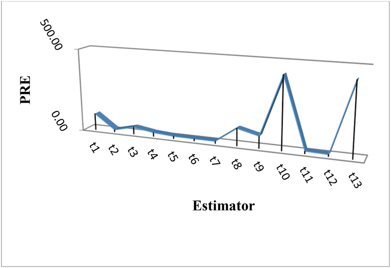
怎么读这张图:分层随机抽样场景下,横轴为样本量 n,纵轴为相对效率 PRE(两估计量方差之比)。不同曲线代表不同估计量相对参照估计量的表现,体现有效性这一统计性质:在无偏的前提下,方差越小的估计量越有效——与本节点估计三大性质(无偏性、有效性、一致性)对应。
5️⃣ 面试实战:估计量比较
题:比较两个无偏估计 $\hat\theta_1$ 和 $\hat\theta_2$,若 $Var(\hat\theta_1) < Var(\hat\theta_2)$,哪个更好? 答:在无偏前提下,方差小者更有效(高斯-马尔可夫定理精神)。
题:什么情况下样本中位数优于样本均值? 答:存在重尾或离群值时,中位数稳健(breakdown point 50%)。
import numpy as np
# 模拟对比:含离群值时,中位数估计位置更稳
rng = np.random.RandomState(41)
x = rng.normal(0, 1, 200)
x_with_outlier = x.copy()
x_with_outlier[0] = 50  # 一个离群值
print('均值: %.3f → %.3f(被拉偏)' % (x.mean(), x_with_outlier.mean()))
print('中位数: %.3f → %.3f(稳健 ✅)' % (np.median(x), np.median(x_with_outlier)))
assert abs(x_with_outlier.mean() - x.mean()) > 0.18 and abs(np.median(x_with_outlier) - np.median(x)) < 0.05
print('✅ 离群值下中位数更稳健')
均值: -0.030 → 0.221(被拉偏)
中位数: 0.001 → 0.025(稳健 ✅)
✅ 离群值下中位数更稳健
🧮 手算示例:指数 MLE 与置信区间逐步算
① 指数 MLE:观测 $[0.5, 1.2, 2.1, 3.4]$(均值 1.8): $$\hat\lambda = \frac{1}{\bar x} = \frac{1}{1.8} \approx 0.5556$$
② 正态均值 95% 置信区间:$[9.8, 10.2, 10.1, 9.9, 10.0]$,已知 σ=0.2,n=5: $$\bar x = 10.0,\quad SE = \frac{0.2}{\sqrt 5} \approx 0.0894$$ $$CI = 10.0 \pm 1.96 \times 0.0894 = [9.825,\; 10.175]$$
import numpy as np
# ① 指数 MLE
x = np.array([0.5, 1.2, 2.1, 3.4])
lam_hat = 1 / x.mean()
print('① 指数 MLE λ̂ =', round(lam_hat, 4), '(手算≈0.5556)')
# ② 正态 CI
y = np.array([9.8, 10.2, 10.1, 9.9, 10.0])
from scipy import stats as st
se = 0.2 / np.sqrt(5)
lo, hi = y.mean() - 1.96*se, y.mean() + 1.96*se
print('② 均值 =', y.mean(), ' SE =', round(se, 4))
print('   CI = [%.3f, %.3f](手算 [9.825, 10.175])' % (lo, hi))
assert abs(lam_hat - 0.5556) < 1e-3
assert abs(lo - 9.8247) < 1e-2 and abs(hi - 10.1753) < 1e-2
print('✅ 手算示例验证通过')
① 指数 MLE λ̂ = 0.5556 (手算≈0.5556)
② 均值 = 10.0  SE = 0.0894
   CI = [9.825, 10.175](手算 [9.825, 10.175])
✅ 手算示例验证通过
✅ 自测清单
- 能说出无偏/有效/一致三性质并用模拟验证 n-1
- 能手推正态/泊松/指数/伯努利的 MLE
- 能解释矩估计与 MLE 的关系
- 能构造正态总体均值的 z 置信区间
- 能讲清 95% CI 的频率解释与常见误区
- 能对比均值/中位数的稳健性